Session 8 – notes
Here are some resources for the Thursday lecture in week 4. I spent most of the time going through the slides and working though some examples – you can see the slides here. Unfortunately the document camera was broken, so I had to draw on the blackboard – I've used some paper sketches below instead.
BCNF, repetition
We started with a retake of one of the problems from last time: we normalized the relation
===========================================
movies(title, year, length, category, star)
-------------------------------------------
fd1: title year star -> length category
fd2: title year -> length category
key: title year star
===========================================
into
=========================================
movie_data(title, year, length, category)
-----------------------------------------
fd: title year -> length category
key: title year
=========================================
and
==============================
movie_stars(title, year, star)
------------------------------
fd: {}
key: title year star
==============================
Both of these are in BCNF, and we discussed at some length why, what it meant, and how to get there (see slides). We also tried this out in the notebook (you can download it and then run jupyter lab, or jupyter notebook – observe that notebooks are JSON files, if you save them with a .ipynb extension, jupyter can run them).
Exercise: Why two attribute relations always are in BCNF
We then proved that two-attribute relations, R(A,B), always are in BCNF. We did it by looking at what functional dependencies we might have:
- None: in this case we're in BCNF by default, since there's no FD which can break BCNF.
A -> B: in this case our key isA, and our only FD has a left hand side which is a superkey.B -> A: in this case our key isB, and our only FD has a left hand side which is a superkey.A -> BandB -> A: in this case we have two candidate keys:AandB, and both our FD's have left hand sides which are superkeys, so we're in BCNF.
QED.
Reconstruction
We then talked about reconstruction – the most important aspect of the algorithm we use for normalizing into BCNF, apart from producing relations in BCNF, is that we can easily reconstruct our original table by joining our new tables using the left hand sides of the FD's we've used to deconstruct.
We looked at an exercise:
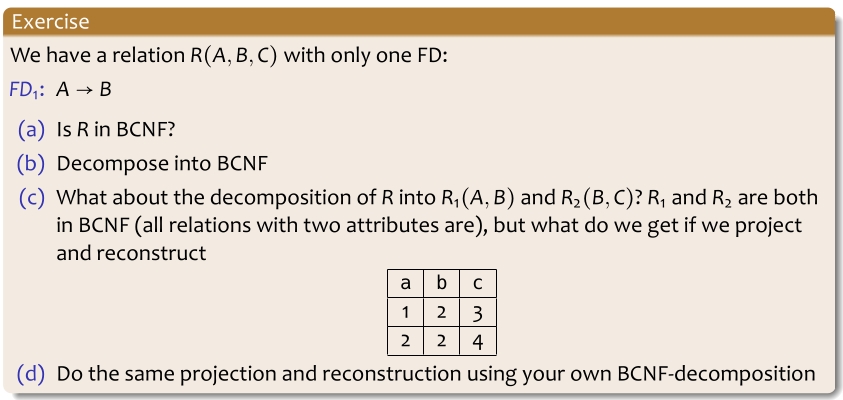
This is what I scribbled on the blackboard
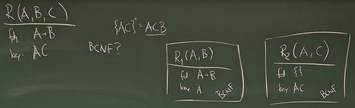
So, using
==============================
R1(A,B)
------------------------------
fd: A -> B
key: A
==============================
and
==============================
R2(A,C)
------------------------------
fd: -
key: AC
==============================
should work.
We tried it in the notebook, where we had the table
| R | A | B | C |
|---|---|---|---|
| 1 | 2 | 3 | |
| 2 | 2 | 4 |
which can be implemented as:
DROP TABLE IF EXISTS R;
CREATE TABLE R (
  a   INT,
  b   INT,
  c   INT
);

INSERT
INTO   R(a,b,c)
VALUES (1,2,3),
       (2,2,4);
To create R1 and R2 from above, we can run:
CREATE TABLE R1 AS
SELECT DISTINCT a, b
FROM   R;
CREATE INDEX r1key ON R1(a);

CREATE TABLE R2 AS
SELECT DISTINCT a, c
FROM   R;
giving:
| R1 | a | b |
|---|---|---|
| 1 | 2 | |
| 2 | 2 |
| R2 | a | c |
|---|---|---|
| 1 | 3 | |
| 2 | 4 |
and then recombine them into one table:
SELECT    a, b, c
FROM      R1
          JOIN R2 USING (a)
which returns:
| a | b | c |
|---|---|---|
| 1 | 2 | 3 |
| 2 | 2 | 4 |
This is an exact replica of the table we started with!
We also tried the ad-hoc decomposition:
==============================
R1(A,B)
------------------------------
fd: A -> B
key: A
==============================
and
==============================
R2(B,C)
------------------------------
fd: -
key: BC
==============================
As we saw above, these relations will both be in BCNF by virtue of being two-attribute relations, but since we haven't used our BCNF-decomposition recipe, we have no guarantee that we can reconstruct our original relation.
We can create the table R2 using:
CREATE TABLE R2 AS
SELECT DISTINCT b, c
FROM   R;
and it will be:
| R2 | b | c |
|---|---|---|
| 2 | 3 | |
| 2 | 4 |
We then tried to join it with R1:
SELECT    a, b, c
FROM      R1
          JOIN R2 USING (b)
and got:
| a | b | c |
|---|---|---|
| 1 | 2 | 3 |
| 1 | 2 | 4 |
| 2 | 2 | 3 |
| 2 | 2 | 4 |
which is not at all what we started out with!
So, using other decompositions than that which our algorithm gives us can result in tables which we can't reconstruct into our original table.
A few words on 3NF, and keeping FD's
We've seen that there are several Normal Forms, and sometimes 3NF can be useful – if we accept tables which are in 3NF, but not all the way into BCNF, we can sometimes keep FD's which can't be kept in BCNF, see the notebook for an example (the bookings table).
More normal forms
Some of the slides towards the end discuss 4NF, which is a generalization of BCNF, where we use multivalued dependencies instead of functional dependencies – we want you to be aware of 4NF, but we won't use it in the course.
A final example
Near the end, I started to normalize the student application database we've seen since lecture 2, we started out with one big table, and identified the functional dependencies.
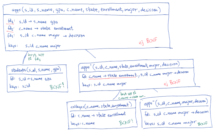
As you can see, the three tables we come up with after the final step, called students, colleges and app'', are the same as the ones we got when we created an ER-model in week 2.
In this case our three final tables happens to contain the same atttributes as our three functional dependencies, but that's 'by coincidence'. Just writing down three relations with the attributes of our functional dependencies will not guarantee that we can reproduce our original relation – only by following our 'recipe' can we be sure to get relations which we can recombine into our original table (on exams, some students just write down relations with the attributes of the functional dependencies, and they may or may not be the same tables we would get if we followed the 'recipe', but a solution without a correct derivation will give zero points, since it gives no guarantee whatsoever that we can recombine our tables into the original).
Earlier we've seen an ER-diagram for the applications:
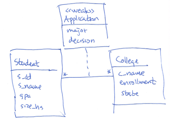
If we translate this into tables, as we did in week 2, we would get exactly the same tables as we got when we normalized into BCNF.